Introduction
In the vast landscape of data science, dealing with high-dimensional datasets is a common challenge. The curse of dimensionality can hinder analysis, introduce computational complexity, and even lead to overfitting in machine learning models. To overcome these obstacles, dimensionality reduction techniques come to the rescue. Among them, Principal Component Analysis (PCA) stands as a versatile and widely used approach.
In this blog, we delve into the world of dimensionality reduction and explore PCA in detail. We will uncover the benefits, drawbacks, and best practices associated with PCA, focusing on its application in the context of machine learning. From the voluntary carbon market, we will extract real-world examples and showcase how PCA can be leveraged to distil actionable insights from complex datasets.
Understanding Dimensionality Reduction
Dimensionality reduction techniques aim to capture the essence of a dataset by transforming a high-dimensional space into a lower-dimensional space while retaining the most important information. This process helps in simplifying complex datasets, reducing computation time, and improving the interpretability of models.
Types of Dimensionality Reduction
- Feature Selection: It involves selecting a subset of the original features based on their importance or relevance to the problem at hand. Common methods include correlation-based feature selection, mutual information-based feature selection, and step-wise forward/backward selection.
- Feature Extraction: Instead of selecting features from the original dataset, feature extraction techniques create new features by transforming the original ones. PCA falls under this category and is widely used for its simplicity and effectiveness.
PCA for Dimensionality Reduction
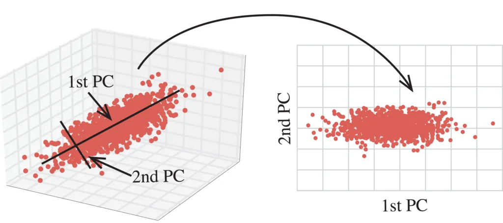
Principal Component Analysis (PCA) is an unsupervised linear transformation technique used to identify the most important aspects, or principal components, of a dataset. These components are orthogonal to each other and capture the maximum variance in the data. To comprehend PCA, we need to delve into the underlying mathematics. PCA calculates eigenvectors and eigenvalues of the covariance matrix of the input data. The eigenvectors represent the principal components, and the corresponding eigenvalues indicate their importance.
Steps for Implementing PCA
- Data Preprocessing: Before applying PCA, it is essential to preprocess the data. This includes handling missing values, scaling numerical features, and encoding categorical variables if necessary.
- Covariance Matrix Calculation: Compute the covariance matrix based on the preprocessed data. The covariance matrix provides insights into the relationships between features.
- Eigendecomposition: Perform eigendecomposition on the covariance matrix to obtain the eigenvectors and eigenvalues.
- Selecting Principal Components: Sort the eigenvectors in descending order based on their corresponding eigenvalues. Select the top k eigenvectors that capture a significant portion of the variance in the data.
- Projection: Project the original data onto the selected principal components to obtain the transformed dataset with reduced dimensions.
Code Snippet: Implementing PCA in Python
# Importing the required libraries
from sklearn.decomposition import PCA
import pandas as pd

# Loading the dataset
data = pd.read_csv('voluntary_carbon_market.csv')

# Preprocessing the data (e.g., scaling, handling missing values)

# Performing PCA
pca = PCA(n_components=2)  # Reduce to 2 dimensions for visualization
transformed_data = pca.fit_transform(data)

# Explained variance ratio
explained_variance_ratio = pca.explained_variance_ratio_
Formula: Explained Variance Ratio The explained variance ratio represents the proportion of variance explained by each principal component.
explained_variance_ratio = explained_variance / total_variance
Scree Plot
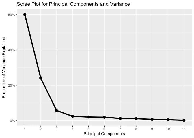
A Visual Aid for Determining the Number of Components One essential tool in understanding PCA is the scree plot. The scree plot helps us determine the number of principal components to retain based on their corresponding eigenvalues. By plotting the eigenvalues against the component number, the scree plot visually presents the amount of variance explained by each component. Typically, the plot shows a sharp drop-off in eigenvalues at a certain point, indicating the optimal number of components to retain.
By examining the scree plot, we can strike a balance between dimensionality reduction and information retention. It guides us in selecting an appropriate number of components that capture a significant portion of the dataset’s variance, avoiding the retention of unnecessary noise or insignificant variability.

Advantages of PCA
- Dimensionality Reduction: PCA allows us to reduce the number of features in the dataset while preserving the majority of the information.
- Feature Decorrelation: The principal components obtained through PCA are uncorrelated, simplifying subsequent analyses and improving model performance.
- Visualization: PCA facilitates the visualization of high-dimensional data by representing it in a lower-dimensional space, typically two or three dimensions. This enables easy interpretation and exploration.
Disadvantages of PCA
- Linearity Assumption: PCA assumes a linear relationship between variables. It may not capture complex nonlinear relationships in the data, leading to a loss of information.
- Interpretability: While PCA provides reduced-dimensional representations, the interpretability of the transformed features might be challenging. The principal components are combinations of original features and may not have clear semantic meanings.
- Information Loss: Although PCA retains the most important information, there is always some loss of information during dimensionality reduction. The first few principal components capture most of the variance, but subsequent components contain less relevant information.
Practical Use Cases in the Voluntary Carbon Market
The voluntary carbon market dataset consists of various features related to carbon credit projects. PCA can be applied to this dataset for multiple purposes:
- Carbon Credit Analysis: PCA can help identify the most influential features driving carbon credit trading. It enables an understanding of the key factors affecting credit issuance, retirement, and market dynamics.
- Project Classification: By reducing the dimensionality, PCA can aid in classifying projects based on their attributes. It can provide insights into project types, locations, and other factors that contribute to successful carbon credit initiatives.
- Visualization: PCA’s ability to project high-dimensional data into two or three dimensions allows for intuitive visualization of the voluntary carbon market. This visualization helps stakeholders understand patterns, clusters, and trends.
Comparing PCA with Other Techniques
While PCA is a widely used dimensionality reduction technique, it’s essential to compare it with other methods to understand its strengths and weaknesses. Techniques like t-SNE (t-distributed Stochastic Neighbor Embedding) and LDA (Linear Discriminant Analysis) offer different advantages. For instance, t-SNE is excellent for nonlinear data visualization, while LDA is suitable for supervised dimensionality reduction. Understanding these alternatives will help data scientists choose the most appropriate method for their specific tasks.
Conclusion
In conclusion, Principal Component Analysis (PCA) emerges as a powerful tool for dimensionality reduction in data science and machine learning. By implementing PCA with best practices and following the outlined steps, we can effectively preprocess and analyze high-dimensional datasets, such as the voluntary carbon market. PCA offers the advantage of feature decorrelation, improved visualization, and efficient data compression. However, it is essential to consider the assumptions and limitations of PCA, such as the linearity assumption and the loss of interpretability in transformed features.
With its practical application in the voluntary carbon market, PCA enables insightful analysis of carbon credit projects, project classification, and intuitive visualization of market trends. By leveraging the explained variance ratio, we gain an understanding of the contributions of each principal component to the overall variance in the data.
While PCA is a popular technique, it is essential to consider other dimensionality reduction methods such as t-SNE and LDA, depending on the specific requirements of the problem at hand. Exploring and comparing these techniques allows data scientists to make informed decisions and optimize their analyses.
By integrating dimensionality reduction techniques like PCA into the data science workflow, we unlock the potential to handle complex datasets, improve model performance, and gain deeper insights into the underlying patterns and relationships. Embracing PCA as a valuable tool, combined with domain expertise, paves the way for data-driven decision-making and impactful applications in various domains.
So, gear up and harness the power of PCA to unleash the true potential of your data and propel your data science endeavours to new heights!
