Machine learning is a powerful tool that allows us to create models capable of making predictions and providing insights from data. However, developing a machine learning model is a complex process that involves various steps, such as data cleaning, feature selection, model building, and evaluation. Model evaluation is an essential step in the machine learning workflow, as it allows us to understand the strengths and weaknesses of our models and guide us in making improvements.

In this post, we’ll cover the key concepts and techniques involved in model evaluation, including evaluation metrics and cross-validation. We’ll also discuss how these concepts apply to classification and regression problems.

Evaluation Metrics for Classification Problems

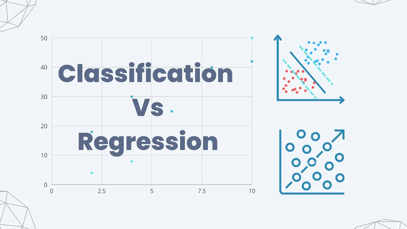
Classification is a type of machine learning problem where the goal is to predict the class labels of new observations based on a set of input features. In other words, given a set of input features, a classifier assigns each observation to one of the predefined classes. For example, a classification model might predict whether a given email is spam or not, based on features such as the sender’s email address, the email’s subject line, and the content of the email.

Evaluation metrics for classification problems help us assess how well our model is performing in predicting these class labels. These metrics quantify the number of correct and incorrect predictions made by the classifier and can be used to compare the performance of different classifiers on the same data set.

Some commonly used evaluation metrics for classification problems include accuracy, precision, recall, F1 score, and area under the receiver operating characteristic (ROC) curve.

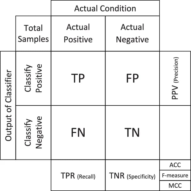
When evaluating the performance of a classifier, we need to consider the number of true positives (TP), true negatives (TN), false positives (FP), and false negatives (FN). These terms are used to describe the results of a binary classification task, where we have two possible classes: positive and negative.

• A true positive (TP) is an observation that is truly positive and is correctly classified as positive by the model. In other words, the model correctly identifies the positive case.
• A true negative (TN) is an observation that is truly negative and is correctly classified as negative by the model. In other words, the model correctly identifies the negative case.
• A false positive (FP) is an observation that is actually negative but is incorrectly classified as positive by the model. In other words, the model incorrectly identifies the negative case as positive.
• A false negative (FN) is an observation that is actually positive but is incorrectly classified as negative by the model. In other words, the model incorrectly identifies the positive case as negative.

Accuracy

Accuracy is a commonly used evaluation metric for classification problems, which measures the proportion of correctly classified observations over the total number of observations. In other words, it tells us how often the classifier correctly predicted the true class label. Mathematically, it can be represented as:

accuracy = (number of correct predictions) / (total number of predictions)

accuracy = (TP + TN) / (TP + TN + FP + FN)

However, accuracy can be misleading when the classes are imbalanced, meaning that one class has significantly more or fewer observations than the other. For example, if we have a data set with 90% of the observations belonging to one class and only 10% belonging to the other, a classifier that always predicts the majority class would achieve an accuracy of 90%, even though it is not predicting the minority class at all.

In such cases, other evaluation metrics such as precision, recall, and F1 score may provide a more accurate picture of the classifier’s performance. These metrics take into account the number of true positives, false positives, true negatives, and false negatives, and are especially useful in imbalanced data sets.

Precision and Recall

Precision and recall are two other evaluation metrics commonly used for classification problems.

• Precision is the proportion of true positive predictions (correctly predicted positive instances) over the total number of positive predictions (both true positives and false positives). It is a measure of how many of the positive predictions are actually correct and is useful when the cost of false positives is high.
• Recall is the proportion of true positive predictions over the total number of actual positive instances in the data set. It is a measure of how many of the actual positive instances the classifier was able to identify and is useful when the cost of false negatives is high.

Mathematically, they can be represented as:

precision = true positives / (true positives + false positives)

recall = true positives / (true positives + false negatives)

Precision and recall are especially useful when dealing with imbalanced datasets, as they provide a more nuanced view of a model’s performance than accuracy.

F1 Score

The F1 score is a commonly used evaluation metric for classification problems, especially when the classes are imbalanced. It is the harmonic mean of precision and recall, which are two important metrics used to evaluate the performance of a binary classifier.

The F1 score combines both precision and recall into a single score, which can be useful when we want to balance the trade-off between these two metrics. A high F1 score indicates that the model is performing well in terms of both precision and recall, while a low F1 score suggests that the model is struggling to correctly identify positive cases.

In situations where precision and recall are equally important, the F1 score can be a useful metric to optimize for.

It can be represented as:

F1 score = 2 * (precision * recall) / (precision + recall)

The F1 score is useful when we want to find a balance between precision and recall.

AUC-ROC Score

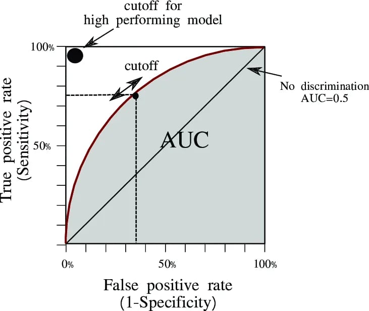
The AUC-ROC score is a widely used evaluation metric for classification problems, particularly in binary classification problems. It measures the area under the receiver operating characteristic (ROC) curve, which is a plot of the true positive rate (TPR) against the false positive rate (FPR) for different classification thresholds.

True Positive Rate (TPR) = TP / (TP + FN)

False Positive Rate (FPR) = FP / (FP + TN)

The ROC curve is generated by varying the classification threshold of a model and plotting the resulting TPR and FPR values at each threshold. The TPR represents the proportion of positive cases that are correctly identified by the model, while the FPR represents the proportion of negative cases that are incorrectly classified as positive by the model.

The AUC-ROC score provides a measure of how well a model can distinguish between positive and negative cases. A perfect model would have an AUC-ROC score of 1, indicating that it has a high TPR and a low FPR, meaning that it correctly identifies most positive cases while making few false positive predictions. A random model, on the other hand, would have an AUC-ROC score of 0.5, indicating that it performs no better than random guessing.

The AUC-ROC score is a useful metric for comparing the performance of different models and selecting the best one for a particular problem. However, like all evaluation metrics, it has its limitations and should be used in conjunction with other metrics to get a comprehensive understanding of a model’s performance.

Evaluation Metrics for Regression Problems

Regression is a supervised learning technique used to predict a continuous output variable based on a set of input features. In regression, the goal is to minimize the difference between the predicted and actual output values.

Evaluation metrics for regression problems are used to measure the performance of the model in predicting the continuous output variable. There are several commonly used evaluation metrics for regression problems, including Mean Absolute Error (MAE), Mean Squared Error (MSE), Root Mean Squared Error (RMSE), and R-squared (R²).

Mean Absolute Error (MAE)

The mean absolute error (MAE) is a commonly used evaluation metric for regression problems. It measures the average absolute difference between the predicted and true values. Mathematically, it can be represented as:

MAE = (1/n) * ∑|yi - ŷi|

Where:

• n is the number of observations
• yi is the actual value
• ŷi is the predicted value

Mean Squared Error (MSE) and Root Mean Squared Error (RMSE)

The mean squared error (MSE) and root mean squared error (RMSE) are other commonly used evaluation metrics for regression problems. MSE measures the average squared difference between the predicted and true values, while RMSE measures the square root of the mean squared error.

Mathematically, they can be represented as:

MSE = (1/n) * Σ(yᵢ - ŷᵢ)²

RMSE = sqrt(MSE)

where:

• n = number of observations
• yᵢ = true value of the i-th observation
• ŷᵢ = predicted value of the i-th observation

Both MSE and RMSE give higher weights to larger errors, which can be useful if we want to penalize large errors more than small errors. However, they may not be appropriate if we want to focus more on the magnitude of the errors rather than their squared values.

Another important point to note is that both MSE and RMSE are sensitive to outliers, as they give more weight to larger errors. Thus, it is important to check for outliers in the data before using these metrics for evaluation.

Cross-Validation

Cross-validation is a technique used to estimate how well a model will perform on unseen data. In cross-validation, the data is split into multiple subsets or folds, and the model is trained on a portion of the data while using the remaining data for validation. The process is repeated multiple times, with each subset serving as a validation set. The results are then averaged to get a more accurate estimate of the model’s performance.

There are several types of cross-validation techniques, including:

1. K-fold cross-validation: In this technique, the data is divided into K equal-sized folds. The model is trained on K-1 folds and validated on the remaining fold. This process is repeated K times, with each fold serving as the validation set once. The average performance across all k folds is then used as the final evaluation metric.
2. Leave-one-out cross-validation: In this technique, the model is trained on all the data except for one observation, which is used for validation. This process is repeated for each observation, and the results are averaged to get a more accurate estimate of the model’s performance.
3. Stratified cross-validation: This technique is used when the data is imbalanced, i.e., the classes are not represented equally. In stratified cross-validation, the data is divided into folds in such a way that each fold contains a representative proportion of each class.

Cross-validation helps to address the problem of overfitting, which occurs when a model is too complex and fits the training data too closely, resulting in poor performance on new, unseen data. By validating the model on multiple subsets of the data, cross-validation helps to ensure that the model generalizes well to new data.

Overall, cross-validation is a powerful technique that can help improve the accuracy and generalization of machine learning models. It is important to carefully choose the appropriate type of cross-validation technique based on the specific characteristics of the data and the modelling problem.

Conclusion

Model evaluation is a critical step in the machine learning workflow that allows us to understand the performance of our models and guide us in making improvements. In this post, we covered the key concepts and techniques involved in model evaluation, including evaluation metrics and cross-validation. We also discussed how these concepts apply to classification and regression problems.

By understanding these concepts and using them to evaluate our models, we can build more accurate and robust machine-learning models that provide valuable insights and predictions from data.